Subsections

• Gauging Definitions
• Measuring Cross-Sectional Area
• Measuring Velocity
  • Using the Flowmeter
  
  
• How Real-Time Stream Gauges Work

Gauging Background

Stream gauging is performed to accurately determine the volume of water moving past a given point per time. This information is crucial for flood planning and prevention, as well as prediction of sediment or contaminant transport, total contaminant or sediment load, prediction and control of erosion, etc. The U.S. Geological Survey maintains a number of real-time stream gauging sites in the U.S. (accessible online) for these purposes.

N. Fork Trinity River at McKinney

The nearest such gauge is near the Heard Museum at McKinney. Click here to see this month's data, see Fig. 3.1 for last two-year's discharge

Map of Texas Gauges

Map showing current surface water summary and station locations for Texas

Mississippi River at Baton Rouge

Gauge height data for last 30 days. Note that maximum annual discharge averages 300,000 cubic ft/sec (cfs).

Map of US Real-Time Data

Map showing current surface water summary and station locations for U.S.

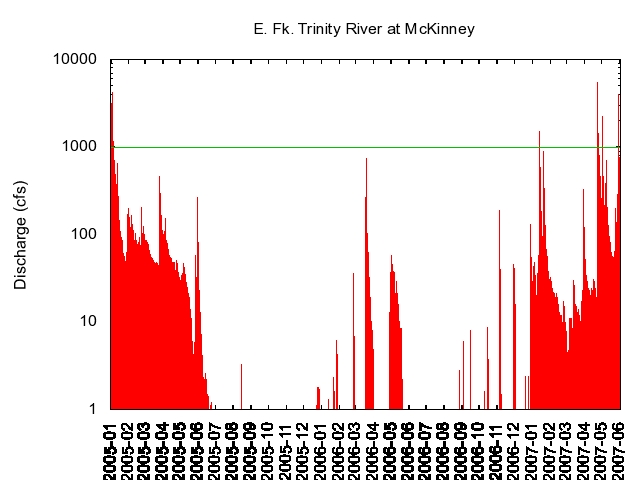
Figure 3.1: Discharge, East Fork Trinity River at McKinney Jan. 2005-May 2007. Heard wetlands fill whenever Trinity discharge exceeds 1000 cfs (horizontal line).

Gauging Definitions

Discharge

is the volume per unit time that passes any point in a stream. Direct measurement of discharge is not possible, but must be calculated from velocity and cross-sectional area of the stream, i.e. from the Discharge Equation

$$\underbrace{Q \left(\mbox{$\rm\frac{L^3}{t}$}\right)}_{\rm... ...} \cdot \underbrace{A (\rm L^2)}_{\rm Cross-Sectional Area}$$ (3.1)

Velocity

is the rate of water movement (Fig. 3.7), but doesn't specify how much (volume of) water is moving. The volume rate is needed to determine flooding, etc.

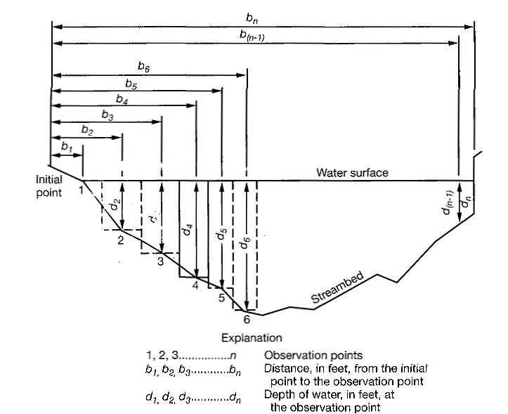
Cross-sectional Area

is the area on a vertical plane cutting the stream (Fig. 3.2)

Stage

is the elevation of the river above its bed, i.e. water depth

You've had direct experience with discharge when using a garden hose with a nozzle. For a given faucet setting (constant input discharge) water shoots farther out of the end of the hose (has higher velocity) when a the nozzle is narrowed (cross-sectional area is reduced). Velocity varies along a stream because of changes in cross-sectional area, but discharge varies only if there is addition or removal of water (e.g. tributaries, evaporation, etc.)

Measuring Cross-Sectional Area

The simplest approach to measuring cross-sectional area is to locate a number of points on the stream bottom by measuring down from the tagline (or yardstick) at regular intervals (see ``$d_i$'' in Fig. 3.2. Then draw these locations (and the water surface) to scale on graph paper, and count the squares to determine the area. A second method is to approximate the area by a series of rectangles, as shown in Fig. 3.2 and Table 3.2, Sanders (1998). If you measure depth at regular intervals (e.g. 2 cm), then the width $b_i$ of each rectangle is constant.

Figure 3.2: Measurement of stream cross-sectional area (after Fig. 3.21, Sanders, 1998).

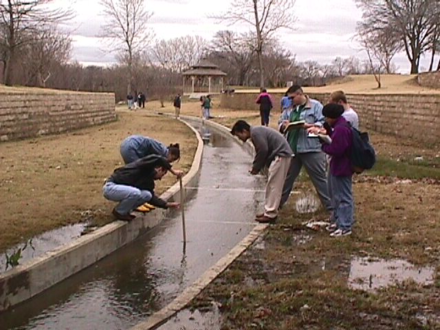
Figure 3.3: Students gauging Cottonwood Creek, UTD. When creek is ``bankfull'' taglines will be used (as shown), when creek is low, yardsticks will replace the taglines and centimeter rulers will be used to measure depths.

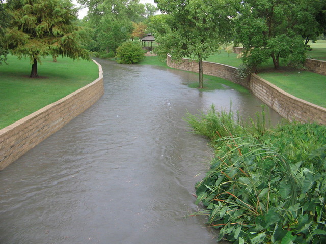
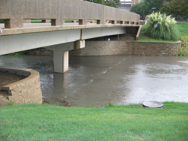
Figure 3.4: Looking downstream from bridge to gazebo, Aug. 15, 2005 flood, taken at 1927h. Larger cross-section of outer channel easily handles storm discharge, culverts at downstream end of channel limit outflow and downstream flooding.

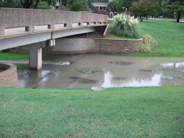
Figure 3.5: Flood recession, Aug.15 2005, looking westward at ``Library'' bridge (stream flowing right to left). Fig. 3.5(b) taken 20 minutes after Fig. 3.5(a), showing designed temporary retention of stormwater by this structure. About 0.5 inches of rain fell in the hour prior to this flood event.

[1926h] [1948h]

Measuring Velocity

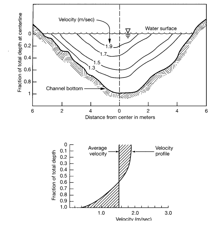
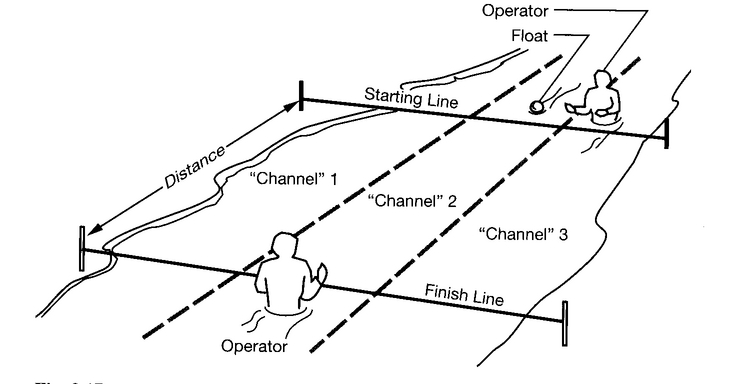
Velocity can be measured directly, using a flowmeter (essentially a speedometer for water, Fig. 3.10 and Section 3.1.3) or inferred by timing the movement of a float in the water (Fig. 3.7). Velocity varies across a stream and with depth, depending primarily on the proximity of the streambed (Fig. 3.6). When using a flowmeter, a single measurement at approximately 60% of the depth of the stream will give a reliable vertical average.

Figure 3.6: Variation of stream velocity with depth (after Fig. 3.16, Sanders, 1998).

Figure 3.7: The float method for velocity determination (after Fig. 3.17, Sanders, 1998).

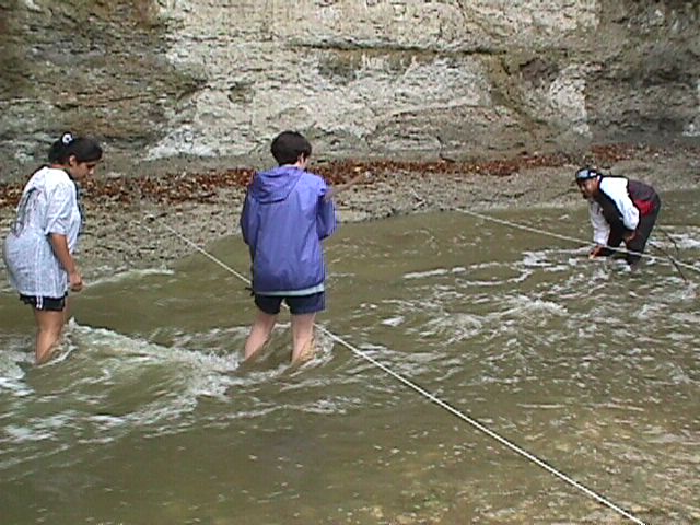
Figure 3.8: Students using the float method for velocity measurement (click on image for full-sized version). Fall '98 class, at Spring Creek, Richardson, Texas.

Using the Flowmeter

The flowmeter can be used to determine average velocity at a point, or across the entire stream (for small streams). The device is waterproof, but try to avoid submerging the LCD display. To use the flowmeter to measure stream velocity:

1. make sure the prop turns freely
2. note the measurement units, ``mi'' on the lower right side of the display denotes english (ft/sec) units, ``km'' denotes metric (m/sec)
3. point the prop directly along the flow, with the black arrow on the prop housing pointing downstream (with the flow). The prop should be fully submerged.
4. press the right button until ``V'' (velocity) appears The instantaneous velocity (in meters/sec) is displayed as the top number on the LCD screen.
5. press the left button to set the lower display to ``av'' for average velocity (initially this number is the maximum ``mx'' velocity)
6. press and hold both left and right buttons simultaneously for 2 seconds to zero the display, and start measurement
7. for point measurements, hold in the flow until the average velocity is constant, then remove the probe. Measurement (averaging) ceases when the prop stops turning, so the displayed value is the true average at the point.
8. for areal measurements (average velocity over a stream cross-section) move the probe in the flow in a steady back-and-forth motion, as if you were spray-painting. When the entire cross-section has been covered, remove the probe from the flow, and record the displayed value.

Figure 3.9: Impeller flowmeter. After http://www.globalw.com/graphics/flow.jpg.

Figure 3.10: Students using an impeller flowmeter (click on image for full-sized version). Fall '98 class, at Spring Creek, Richardson, Texas.

How Real-Time Stream Gauges Work

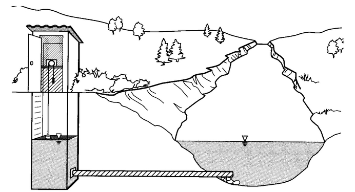
The links in Section 3.1 show up-to-the-minute discharge at USGS and Army Corp of Engineers stream gauges. The procedure described above is too cumbersome to provide such data, instead it is derived from constant stream level (stage) monitoring using ``Stilling wells'' (Fig. 3.11), from which discharge is estimated using a ``rating curve'' (Fig. 3.12) for that site. The rating curve is derived by using the procedure we'll use in this lab for a variety of discharge levels.

Figure 3.11: Schematic of stream water level monitoring station (after Fig. 3.17, Sanders, 1998). The configuration shown is known as a ``Stilling well'', most stations simply have a PVC tube in place of the well.

Figure 3.12: Example rating curve for a stream gauging station (after Fig. 3.22, Sanders, 1998). Given measurements of discharge at various river levels (stage), the rating curve can be obtained and used to estimate dischage given a stage measurement.x