To investigate the eigenvalue spectrum of the Liouville operator
subject to the boundary conditions (4.36) we again construct
a small, discrete model. The position variable q will take the same
set of discrete values that x did in the previous section:
 .
The values of p are also restricted to a discrete, bounded set:
.
The values of p are also restricted to a discrete, bounded set:
 . The mesh spacing in the p
direction is thus
. The mesh spacing in the p
direction is thus  . The choice of the discrete
values for p follows from a desire to avoid the point p = 0 and the
need to satisfy a Fourier completeness relation, which will be discussed
later. The discrete Wigner distribution is then related to the discrete
density matrix of Section 3.2 by
. The choice of the discrete
values for p follows from a desire to avoid the point p = 0 and the
need to satisfy a Fourier completeness relation, which will be discussed
later. The discrete Wigner distribution is then related to the discrete
density matrix of Section 3.2 by
where j indexes position q, and k indexes momentum p.
The discrete version of the potential term is readily defined. Using (4.42) the discrete potential kernel becomes
[Notice
that (4.43) invokes values of  which are outside the
domain
which are outside the
domain  . This expresses the
nonlocality of quantum phenomena and is one way in which the environment
of an open system influences the system's behavior. The values which
one assumes for
. This expresses the
nonlocality of quantum phenomena and is one way in which the environment
of an open system influences the system's behavior. The values which
one assumes for  , where
  or
or  , depend upon the
nature of the environment. If ideal reservoirs are assumed, then
setting these values equal to the potential at the appropriate boundary
appears to be an adequate procedure.] The
elements of
, depend upon the
nature of the environment. If ideal reservoirs are assumed, then
setting these values equal to the potential at the appropriate boundary
appears to be an adequate procedure.] The
elements of  are then:
where the notation  is introduced to shorten the expressions to be derived from the discrete
Liouville equation.
Note that the elements of
is introduced to shorten the expressions to be derived from the discrete
Liouville equation.
Note that the elements of  are real and that
 so
so  is an imaginary Hermitian superoperator.
The boundary conditions (4.36) affect the form of the drift
term  because they determine the proper finite-difference form
for the gradient. On a discrete mesh a first derivative
because they determine the proper finite-difference form
for the gradient. On a discrete mesh a first derivative  can be approximated by either a left-hand difference
or a right-hand difference
(There is also a centered difference form,  , which has poor stability properties when used to approximate a
drift term.) The boundary conditions
determine which of the above difference forms must be used simply
because one or the other will not couple the boundary value into the
domain. Again, let us imagine that the boundary conditions
(4.36) are implemented by fixing the value of f on mesh points
just outside the domain:
, which has poor stability properties when used to approximate a
drift term.) The boundary conditions
determine which of the above difference forms must be used simply
because one or the other will not couple the boundary value into the
domain. Again, let us imagine that the boundary conditions
(4.36) are implemented by fixing the value of f on mesh points
just outside the domain:
This scheme is illustrated in Fig. 8.
Figure 8. Discretization scheme for the kinetic-energy superoperator (drift term)Considerin the Wigner representation. The flow of probability between mesh points is indicated by the arrows, which also define the sense of the finite-difference approximation for the gradient. A flow toward the right requires a left-hand difference and vice versa. This is the ``upwind'' difference scheme and is uniquely determined by the form of the boundary conditions (4.36).
 .
The boundary conditions are specified for
.
The boundary conditions are specified for  , and if this value
is to be coupled into the domain, we must use the left-hand difference
formula (4.45) for the gradient at
, and if this value
is to be coupled into the domain, we must use the left-hand difference
formula (4.45) for the gradient at  . Consistency then
requires that we use the left-hand difference for all
. Consistency then
requires that we use the left-hand difference for all  (for
(for  ).
Similarly, we must use the right-hand difference (4.46) for
).
Similarly, we must use the right-hand difference (4.46) for  .
In the context of hydrodynamic calculations such a difference scheme is
called an ``upwind'' or ``upstream'' difference and is known to
enormously enhance the stability of a computation (Roache, 1976, pp
4--5). It
has also been used in neutron transport calculations at the kinetic
(phase space) level (Duderstadt and Martin, 1979).
The elements of
.
In the context of hydrodynamic calculations such a difference scheme is
called an ``upwind'' or ``upstream'' difference and is known to
enormously enhance the stability of a computation (Roache, 1976, pp
4--5). It
has also been used in neutron transport calculations at the kinetic
(phase space) level (Duderstadt and Martin, 1979).
The elements of  are thus:
The terms  and
and  couple to
the fixed boundary values of f and are thus the coefficients of
inhomogeneous terms and are not strictly elements of
couple to
the fixed boundary values of f and are thus the coefficients of
inhomogeneous terms and are not strictly elements of  . (In
particular, these terms are not included in the eigenvalue calculation
because eigenvalues are properties of homogeneous linear operators.)
It is convenient to group these terms into a boundary contribution
. (In
particular, these terms are not included in the eigenvalue calculation
because eigenvalues are properties of homogeneous linear operators.)
It is convenient to group these terms into a boundary contribution
 :
:
The discrete form of the Liouville equation then becomes
with the inhomogeneous terms explicitly displayed. Expanding the definitions of the operators, the Liouville equation can be written as
This provides a more convenient starting point for many of the manipulations which will be described below.
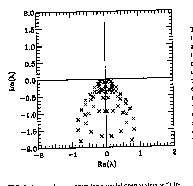
Figure 9. Eigenvalue spectrum for a model open system with irreversible boundary conditions. All eigenvalues have negative imaginary parts, verifying that the model is stable, despite the fact that no damping is yet included.
The eigenvalue spectrum for  constructed from
(4.37), (4.44), and (4.48) is shown in
Fig. 9. The potential of Fig. 4 was
used, with
constructed from
(4.37), (4.44), and (4.48) is shown in
Fig. 9. The potential of Fig. 4 was
used, with  and
and  . All the eigenvalues of
  have negative imaginary parts. (Note in particular that there is no
eigenvalue equal to zero, and thus
have negative imaginary parts. (Note in particular that there is no
eigenvalue equal to zero, and thus  is nonsingular.)
Because the eigenvalues have negative imaginary parts, the
time-dependence of f contains only decaying exponentials, so the model
is stable. The stability of this model follows from the boundary
conditions (4.36) and does not depend upon discretization
(Frensley, 1986). To
demonstrate this, let us consider the expectation value of
is nonsingular.)
Because the eigenvalues have negative imaginary parts, the
time-dependence of f contains only decaying exponentials, so the model
is stable. The stability of this model follows from the boundary
conditions (4.36) and does not depend upon discretization
(Frensley, 1986). To
demonstrate this, let us consider the expectation value of  with respect to an arbitrary distribution f:
  . If we demonstrate that this is
nonpositive for any f, we will have shown that no eigenvalue of
. If we demonstrate that this is
nonpositive for any f, we will have shown that no eigenvalue of
 has a positive real part, because the operator itself is
purely real. In the Wigner-Weyl representation the
operator inner product (2.4) becomes simply
(Wigner, 1971; Hillery, O'Connell, Scully, and Wigner, 1984):
has a positive real part, because the operator itself is
purely real. In the Wigner-Weyl representation the
operator inner product (2.4) becomes simply
(Wigner, 1971; Hillery, O'Connell, Scully, and Wigner, 1984):
The expectation value can be rewritten
because  from the antisymmetry of
 . For the mathematically homogeneous problem (source terms set
to zero) the boundary conditions are
. For the mathematically homogeneous problem (source terms set
to zero) the boundary conditions are
 for p>0 and
  for p<0. With this we can
integrate the expectation value for
for p<0. With this we can
integrate the expectation value for  and simplify it to obtain
Thus, the stability of the solutions to the Liouville equation using
 follow from the boundary conditions alone. The physical
significance of this argument is that the particles in an open system
will eventually escape and the density will approach zero if there is no
inward current flow from the environment. However, if the potential has
a local
minimum within the system deep enough to create one or more
bound states, any particles in those states will not escape. Their
contribution to f will be zero at the boundaries, and this is the
significance of the case in which (4.54) is equal to zero.
Such
states should correspond to eigenvalues of
follow from the boundary conditions alone. The physical
significance of this argument is that the particles in an open system
will eventually escape and the density will approach zero if there is no
inward current flow from the environment. However, if the potential has
a local
minimum within the system deep enough to create one or more
bound states, any particles in those states will not escape. Their
contribution to f will be zero at the boundaries, and this is the
significance of the case in which (4.54) is equal to zero.
Such
states should correspond to eigenvalues of  which are equal to zero,
although I have not observed such a situation in the models
which I have examined. In an open system of finite extent and with
potentials of finite depth, the tunneling tail of a bound-state
wavefunction will be nonzero at the system boundaries, perhaps leading
to a finite rate of escape from that state within the present model.
which are equal to zero,
although I have not observed such a situation in the models
which I have examined. In an open system of finite extent and with
potentials of finite depth, the tunneling tail of a bound-state
wavefunction will be nonzero at the system boundaries, perhaps leading
to a finite rate of escape from that state within the present model.
Let us examine how this open system model can be used. The methods of calculation are more readily visualized if we write (4.50) in a block-matrix notation:
Here  and
and  represent column vectors, and
  and
and  represent matrices, whose internal indices range
over the allowed values of k. The
represent matrices, whose internal indices range
over the allowed values of k. The  are diagonal matrices,
whereas the
are diagonal matrices,
whereas the  are dense. The block-tridiagonal form of
 greatly reduces the computational labor required to solve the
Liouville equation compared to that required to work with superoperators
of a more general form.
greatly reduces the computational labor required to solve the
Liouville equation compared to that required to work with superoperators
of a more general form.
Now suppose that we wish to find
the nonequilibrium steady state ( ).
Can we simply move the
).
Can we simply move the  column vector over
to the other side of the equation and solve for the
column vector over
to the other side of the equation and solve for the  ? The
answer is yes, provided that the operator
? The
answer is yes, provided that the operator  is nonsingular. If
there are no bound states, all the eigenvalues of
is nonsingular. If
there are no bound states, all the eigenvalues of  are nonzero
(see Fig. 9), so
are nonzero
(see Fig. 9), so  is a nonsingular operator and
its inverse exists. This steady-state solution for the
Wigner function may be written:
is a nonsingular operator and
its inverse exists. This steady-state solution for the
Wigner function may be written:
where  refers to the ``direct current'' case. Equation
(4.55) is also used to solve time-dependent problems, as
will be described in the following section.
refers to the ``direct current'' case. Equation
(4.55) is also used to solve time-dependent problems, as
will be described in the following section.
Let us compare this approach to the most commonly studied problem in
transport theory, transport in a spatially homogeneous system with a
uniform driving field (as is done to evaluate transport coefficients
such as mobilities) (Dresden, 1961; Conwell, 1967).
This generates a mathematically homogeneous
problem, and the solution corresponds to the null space of that
superoperator which appears in the transport equation (Aubert,
Vaissiere, and Nougier, 1984).
Thus, the
superoperator must be singular and, if the transport equation is linear,
the solution is not unique (the total density is not determined). What the
present model demonstrates is that this formulation of transport
through a spatially inhomogeneous system leads to a mathematically
inhomogeneous problem, which is in many respects a good deal simpler
than a similar homogeneous problem. For example, because  is
nonsingular, there is no problem of compatibility relations for the
boundary conditions (Lanczos, 1961). Any choice of distribution function
on the boundary will generate a unique steady-state solution. The same
considerations apply to the evaluation of the transient response of an
open system by integrating (4.33) with respect to t. The
solution is unique and, as we have seen, stable.
is
nonsingular, there is no problem of compatibility relations for the
boundary conditions (Lanczos, 1961). Any choice of distribution function
on the boundary will generate a unique steady-state solution. The same
considerations apply to the evaluation of the transient response of an
open system by integrating (4.33) with respect to t. The
solution is unique and, as we have seen, stable.
These considerations clarify a point discussed by Kluksdahl et al. (1989), concerning the role of the initially assumed Wigner function in a calculation in which the steady state is found by simulating the time evolution. Kluksdahl et al. assert that the initial state must be quantum-mechanically correct. The only components of the initial state which remain through the time-evolution calculation are those which lie in the null space of the Liouville operator. All other components will approach steady-state values which are independent of the initial condition. Thus, if there is no null space (the operator is nonsingular) the initial condition makes no difference whatsoever. A concern about the correctness of the initial state is warranted only if there are bound states within the system, and possibly in the continuum limit where the smallest eigenvalue approaches zero.