The steady-state behavior of the RTD has been evaluated using the
Wigner function in an open-system model by several groups
(Frensley, 1986, 1987; Kluksdahl et al., 1988, 1989; Mains and
Haddad, 1988b; Jensen and Buot, 1989a).
To obtain the results described here, the steady-state Wigner function
was evaluated using (4.56) repeatedly for
a set of potentials representing different applied bias voltages. (The
assumed structure consisted of a 4.5 nm GaAs quantum well bounded by 2.8
nm  barrier layers. The contact
layers were assumed to be doped so as to produce a free electron density
of
barrier layers. The contact
layers were assumed to be doped so as to produce a free electron density
of  , and the temperature was taken to be
300 K.) The boundary distribution was taken to be
, and the temperature was taken to be
300 K.) The boundary distribution was taken to be
to include the integration over transverse momenta. [Here  is
evaluated at each boundary using the charge-neutrality
condition (9.131).] The
current density was evaluated from
is
evaluated at each boundary using the charge-neutrality
condition (9.131).] The
current density was evaluated from  , and the resulting
  curve
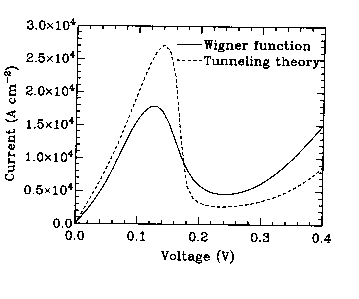
is plotted in Fig. 11. Also shown for comparison is the
result of a more conventional tunneling theory calculation, such as that
described in Appendix 9. [More specifically, it is
the current density that would be obtained by taking the expectation
value of the current operator with respect to the density operator
(9.132).]
curve
is plotted in Fig. 11. Also shown for comparison is the
result of a more conventional tunneling theory calculation, such as that
described in Appendix 9. [More specifically, it is
the current density that would be obtained by taking the expectation
value of the current operator with respect to the density operator
(9.132).]
Figure 11. Current density as a function of voltage for a model resonant-tunneling diode. The result of the time-irreversible kinetic (Wigner function) model is shown by the solid line, and a more conventional tunneling calculation is shown by the dashed line. While they differ in detail, the calculations agree as to the qualitative behavior of the far-from-equilibrium steady state and predict tunneling currents of the same order of magnitude.
The two
calculations agree on the qualitative shape of the  curve and on
the voltages at which the peak and valley occur. There is a
disagreement of some tens of percent on the magnitude of the peak and
valley current. One can cite at least two possible sources of this
disagreement. The more obvious one is that the Wigner-function
calculation necessarily introduces a limited coherence length because
in the discrete approximation the integral defining the nonlocal potential
(4.34) must be cut off at a finite value as in (4.43).
The tunneling theory is based upon solutions of Schrödinger's equation,
which necessarily assumes an infinite coherence length. A second, and
probably more fundamental, explanation for the disagreement is that the
tunneling and kinetic theories are simply not equivalent (the kinetic
theory being Markovian while the tunneling theory is not). The notion
that these theories can be viewed as different approximations to a more
general many-body theory is examined in Sec.
6.3.
curve and on
the voltages at which the peak and valley occur. There is a
disagreement of some tens of percent on the magnitude of the peak and
valley current. One can cite at least two possible sources of this
disagreement. The more obvious one is that the Wigner-function
calculation necessarily introduces a limited coherence length because
in the discrete approximation the integral defining the nonlocal potential
(4.34) must be cut off at a finite value as in (4.43).
The tunneling theory is based upon solutions of Schrödinger's equation,
which necessarily assumes an infinite coherence length. A second, and
probably more fundamental, explanation for the disagreement is that the
tunneling and kinetic theories are simply not equivalent (the kinetic
theory being Markovian while the tunneling theory is not). The notion
that these theories can be viewed as different approximations to a more
general many-body theory is examined in Sec.
6.3.
The Wigner distribution functions which underlie the  curve of
Fig. 11 are illustrated in Figs.
12--14. The equilibrium (zero bias) case is
shown in Fig. 12. The large electron density in the
electrode regions, and much smaller density in the vicinity of the
quantum well, is evident. Fig. 13 shows the Wigner
function for a bias voltage of 0.13 V, which corresponds to the peak of
the resonant-tunneling current. The negative peak indicates that strong
quantum-interference effects are present. In contrast, the Wigner
function for 0.24 V, at the minimum valley current, is quite similar to
the equilibrium case.
curve of
Fig. 11 are illustrated in Figs.
12--14. The equilibrium (zero bias) case is
shown in Fig. 12. The large electron density in the
electrode regions, and much smaller density in the vicinity of the
quantum well, is evident. Fig. 13 shows the Wigner
function for a bias voltage of 0.13 V, which corresponds to the peak of
the resonant-tunneling current. The negative peak indicates that strong
quantum-interference effects are present. In contrast, the Wigner
function for 0.24 V, at the minimum valley current, is quite similar to
the equilibrium case.
Figure 12. Wigner distribution function for the resonant-tunneling diode at zero bias voltage (thermal equilibrium). In the electrode (flat-potential) regions the distribution is approximately Maxwellian (as a function of p). The density is reduced in the vicinity of the quantum well due to size-quantization effects. The very small ripples perceptible at larger p are due to standing waves near the energy barriers.
Figure 13. Wigner distribution function for 0.13 V bias, at the peak of thecurve. The complex standing-wave patterns and prominent negative peak indicate that strong quantum-interference effects are present.
Figure 14. Wigner distribution function for 0.24 V bias, corresponding to the bottom of the valley in thecurve. This case is quite similar to the equilibrium case of Fig. 12.